Area and volume

Consider a bounded object in \(\real^2\). An example is shown in Figure 8. The area, \(A\), of the object can be efficiently estimated by point counting. Onto the object, overlay a test system of points uniform randomly and count the number of test points hitting the object. The sample space or set of all possible outcomes, \(\Omega\), is {0 points hit object, 1 point hits object, 2 points hit object, ...}. Let \(P\) be the random variable \(P(\omega) = \omega\). If the area per test point is \(a/p\), then

$$A = \frac{a}{p} \cdot \mathbf{E}P. \tag{25} $$

An estimate of \(A\) can be obtained from a single throw of the test system of points:

$$\hat{A} = \frac{a}{p} \cdot P. \tag{26} $$

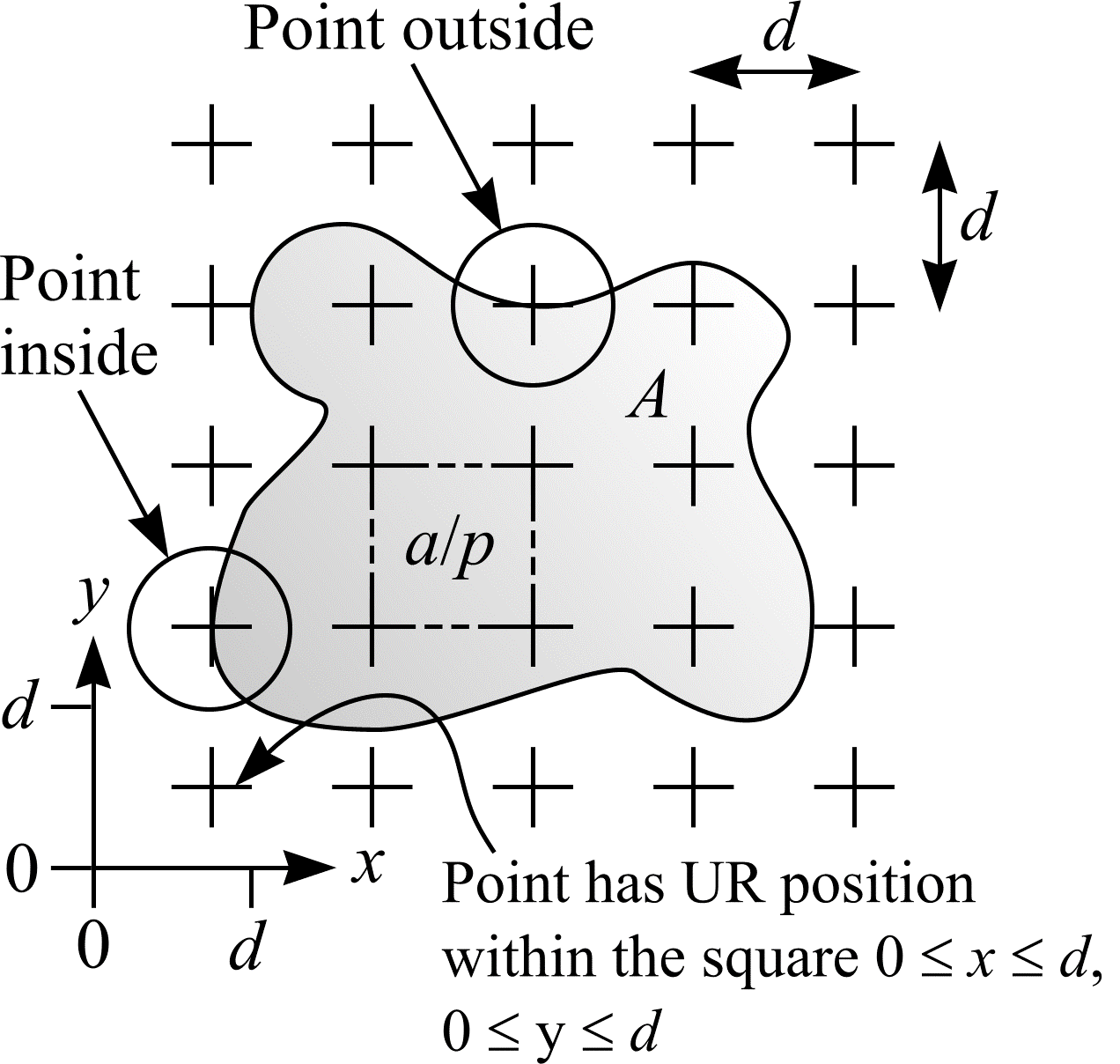
Figure 8: Area estimation using a test system of points. The area per point is \(a/p\). A test point is a zero dimensional probe; to remove the influence of line thickness, Weibel (1979, p.113) defines a test point as the true point of intersection between the upper edge of the horizontal line of a cross, and the right-hand side edge of the vertical line of the cross. In this example, \(P\) = 9.

Now consider a bounded object in \(\real^3\). An example is shown in Figure 9. The volume, \(V\), of the object can be estimated if the object is systematically sampled by plane sections. Fix a convenient axis relative to the object. Next, intersect the object by a Uniform Random (UR) systematic set of parallel planes, a given distance \(T\) apart, and normal to the chosen axis. Let the random variables \(A_{1}\), \(A_{2}\), ..., \(A_{m}\) denote the successive cross-sectional areas formed by the intersection of the bounded object with the parallel planes. If the random variable \(A_{T}\) represents the sum of the cross section areas,

$$V = T \cdot \mathbf{E}A_{T}. \tag{27} $$

An estimate of \(V\) can be obtained from a single throw of the parallel plane test system:

$$\hat{V} = T \cdot \sum_{i=1}^{n} A_{i}. \tag{28} $$

A further approximation of \(V\) is possible if each cross sectional area is estimated with a uniform random grid of points:

$$ \begin{align} \hat{V} &= T \cdot \sum_{i=1}^{n} A_{i} \\ &= T \cdot \frac{a}{p} \cdot \sum_{i=1}^{n} \mathbf{E}P_{i}, \end{align} \tag{29} $$

so that

$$\hat{V_{2}} = T \cdot \frac{a}{p} \cdot \sum_{i=1}^{n} P_{i}. \tag{30} $$

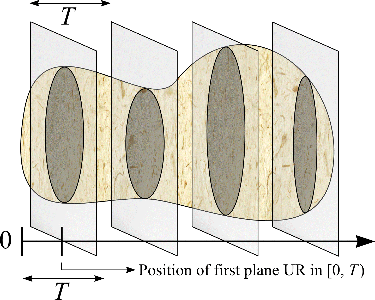
Figure 9: Volume estimation using the Cavalieri method.

This method of volume estimation is called the Cavalieri method. The method is named after the Italian mathematician Bonaventura Cavalieri (1598-1647), a pupil of Galileo. To apply the Cavalieri method without incurring bias, sections have to be truly planar or infinitely thin. If the distance, \(T\), between parallel sections varies, then \(T\) may be replaced with its mean value. There are many examples where the Cavalieri method has been used to estimate volume. Michel and Cruz-Orive (1988) estimated lung volume. Roberts et al. (1993) and (1994) used MRI to estimate, respectively, human body composition and fetal volume.

References

MICHEL, R. P. and CRUZ-ORIVE, L. M. Application of the Cavalieri principle and vertical sections method to lung: estimation of volume and pleural surface area. J. Microsc., 150, 117-136 (1988).

ROBERTS, N., CRUZ-ORIVE, L. M., REID, M., BRODIE, D., BOURNE, M. and EDWARDS, R. H. T. Unbiased estimation of human body composition by the Cavalieri method using magnetic resonance imaging. J. Microsc., 171, 239-253 (1993).

ROBERTS, N., GARDEN, A. S., CRUZ-ORIVE, L. M., WHITEHOUSE, G. H. and EDWARDS, R. H. T. Estimation of fetal volume by MRI and stereology. The British Journal of Radiology, 67, 1067-1077 (1994).

WEIBEL, E. R. Stereological Methods. Vol. 1: Practical Methods for Biological Morphometry. London - New York - Toronto: Academic Press (1979).