Curve length in \(\real^{2}\)

Consider the curve, \(C\), shown in Figure (11). \(C\) can be approximated by \(Y = \bigcup(y_{i})_{i=1}^{n} = \{ y_{1}, y_{2}, ..., y_{i}, ..., y_{n} \}\) (a union of line segments). If the length of \(y_{i}\) is \(b_{i} (1 \le i \le n)\), an approximation of the curve length of \(C\) is \(B = \sum_{i=1}^{n} b_{i}\).

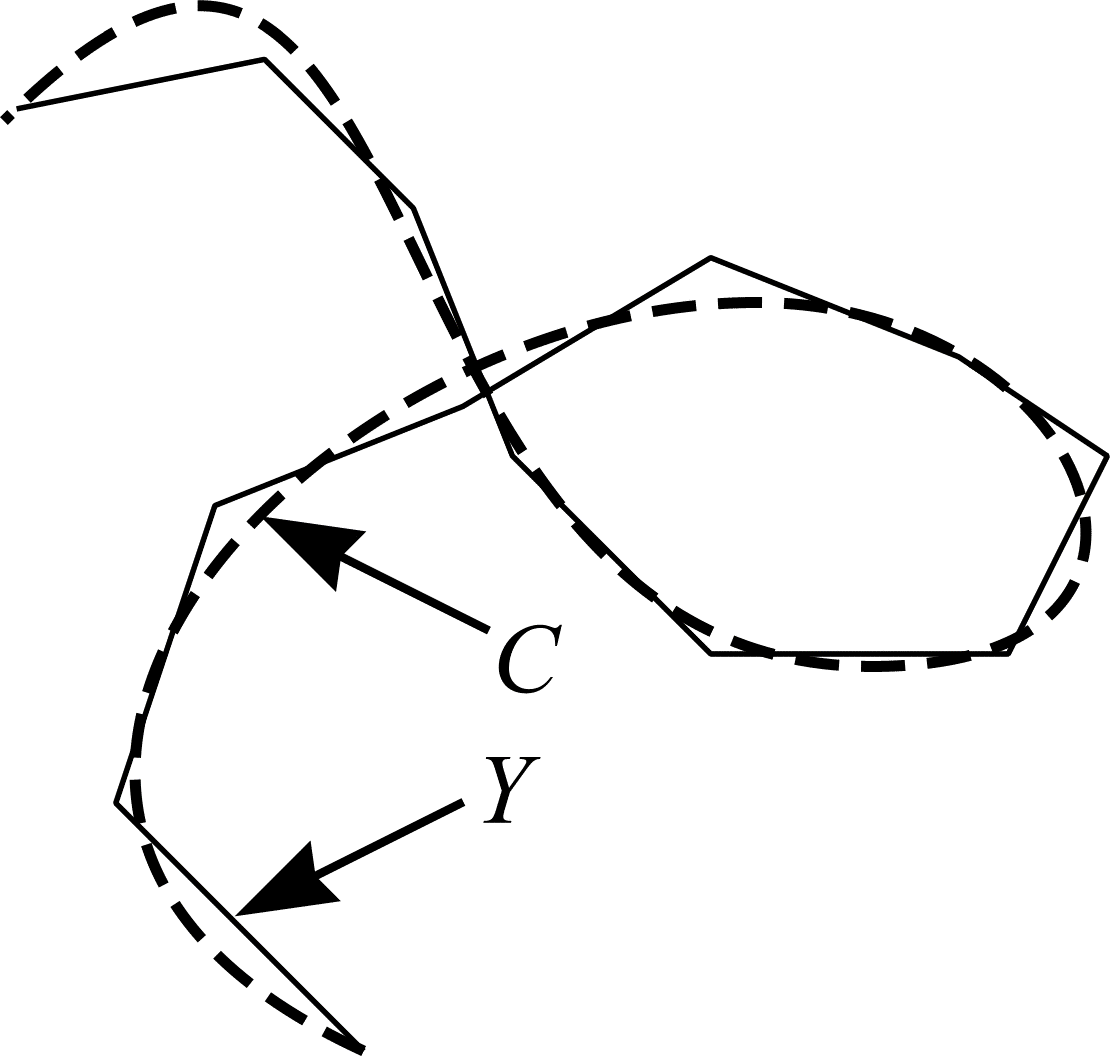
Figure 11: A curve approximated by line segments.

The methodology of Buffon's needle allows the length of each line segment and hence \(B\) to be estimated. Once more, imagine a room whose floor is made up of planks of wood. The planks have uniform width, \(h\) (with \(b_{i} < h)\), and are parallel to one another. \(Y\) is thrown into the air and lands on the floor. \(Y\) is assumed to be IUR in the plane. A sufficient condition for this to be true is that \(y_{1}\) is IUR in the plane. By comparison with (31), the probability that the line segment \(y_{i}\) intersects a joint is \(2b_{i} /\pi h\). Furthermore, (32) implies the length of \(y_{i}\) is \(b_{i} = (\pi / 2) \cdot h \cdot \mathbf{E} I_{i}\). \(I_{i}\) is a discrete random variable that maps the outcomes \(y_{i}\) intersects a joint and \(y_{i}\) falls between joints to the real numbers 1 and 0, respectively. Let the total number of intersections, \(I\), between the joints and \(Y\) be denoted as the sum \(I_{1} + I_{2} + ... + I_{n}\). Taking into account all line segments:

$$ \begin{align} B &= \frac{\pi}{2} \cdot h \cdot \sum_{i=1}^{n} \mathbf{E}I_{i} \\ &= \frac{\pi}{2} \cdot h \cdot \mathbf{E}I. \end{align} \tag{34} $$

An estimate of \(B\) can be obtained from a single throw of \(Y\):

$$ \begin{align} \hat{B} &= \frac{\pi}{2} \cdot h \cdot \sum_{i=1}^{n} I_{i} \\ &= \frac{\pi}{2} \cdot h \cdot I. \end{align} \tag{35} $$

As the number of line segments is increased, the approximation of \(C\) is refined. In the limit \((n \to \infty)\), \(Y\) becomes \(C\) and (34) gives the exact curve length of \(C\).

Consider again the array of joints onto which \(Y\) is randomly thrown. The joints can be thought of as an unbounded, systematic set of parallel test lines a distance \(h\) apart. As such, the average length of test line likely to fall within a certain area can be calculated. Figure 12(a) shows a length of test line, \(L\), and the area it occupies. The test system of lines has length per unit area \(L/A = L/Lh = 1/h\). Next, substitute \(h = A/L\) into (34). The result is a well-known formula originally due to Steinhaus (1930):

$$ \begin{align} \frac{B}{A} &= \frac{\pi}{2} \cdot \frac{\mathbf{E}I}{L} \\ \text{and so } B &= \frac{\pi}{2} \cdot \frac{A}{L} \cdot \mathbf{E}I \end{align} \tag{36} $$

An estimate of \(B\) can be obtained from a single throw of \(Y\):

$$ \hat{B} = \frac{\pi}{2} \cdot \frac{A}{L} \cdot I. \tag{37} $$

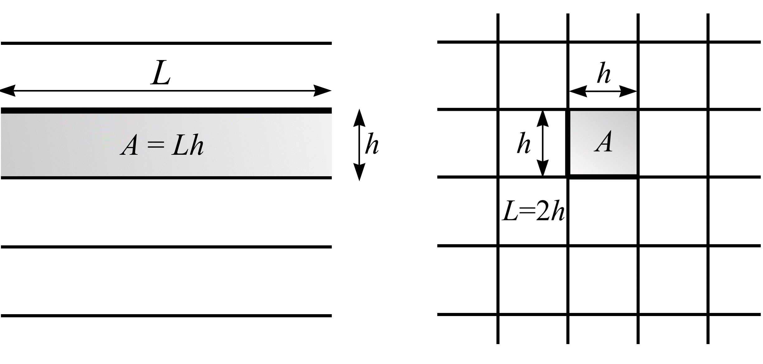
Figure 12: Test systems of (a) parallel lines (\(L/A = 1/h\)) and (b) mutually orthogonal lines (\(L/A = 2/h\)). The figure shows each test system with the area, \(A\), a length of test line, \(L\), occupies.

Suppose a needle, length \(B\) (\(B > h\)), is thrown with IUR position onto a test system of parallel lines. \(\hat{B}\) is greatest when the needle is perpendicular to the test lines and smallest when the needle is parallel to the test lines. A better estimation of \(B\) is obtained if the test system of parallel lines is replaced by a test system of mutually orthogonal lines (see Figure 12(b)). Such a test system has twice as much length per unit area as the parallel line test system so that \(L/A = 2 \cdot (1/h)\).

One way of determining a test system's length per unit area, \(L/A\), is by tiling the plane \((\real^{2})\) with fundamental tile, \(J_{0}\), of known area \(A\) where the mean length of test curve falling within each tile is \(L\). The test line elements of the test systems described in Figure 12 may be rearranged into any arbitrary curve shape whose mean length per unit area, \(L/A\), is known. This is because an IUR test line element is invariant under arbitrary translations and rotations. Therefore, the test system of rolling circles, shown in Figure 13, may be used in place of either of the test systems shown in Figure 12 to estimate curve length in \(\real^{2}\).

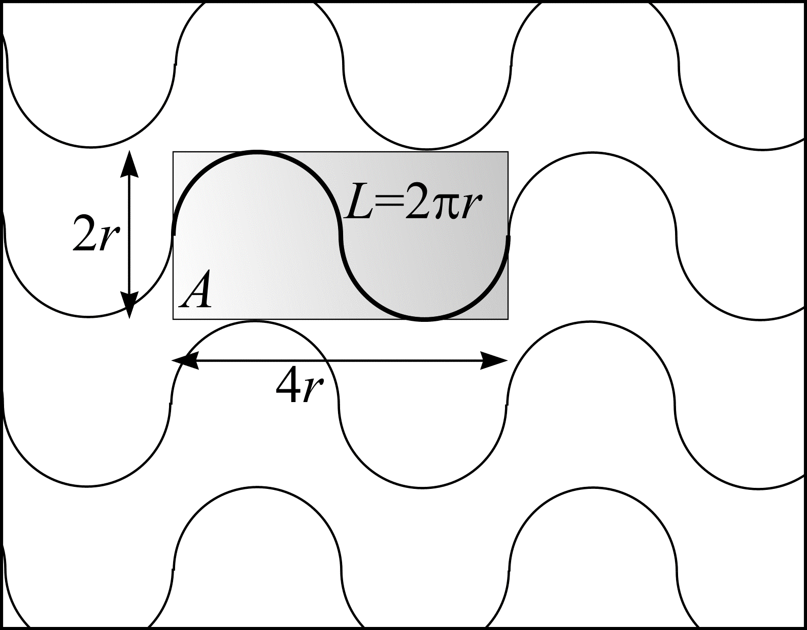
Figure 13: A test system of rolling circles, radius \(r\). The figure shows the area, \(A\), a length of test line, \(L\), occupies. The test system has length per unit area, \(L/A = \pi/4r\).

References

STEINHAUS, H. Zur Praxis der Rektifikation und zum Längenbegriff. Berichte Sächsischen Akad. Wiss. Leipzig, 82, 120-130 (1930).