Continuous random variables
The random variable \(X\) is continuous if its distribution function can be expressed as
$$ \begin{align} F_{X}(x) &= \mathbf{P}(X \le x) \\ &= \int_{-\infty}^{x}f_{X}(u)\mathrm{d}u, & x \in \real, \end{align} \tag{6} $$
for some integrable function \(f_{X} : \real \to [0, \infty)\). In this case, \(f_{X}\) is called the (probability) density function of \(X\). The fundamental theorem of calculus and (6) imply
$$ \begin{align*} \mathbf{P}(a \le X \le b) &= F_{X}(b) - F_{X}(a) \\ &= \int_{a}^{b}f_{X}(x)\mathrm{d}x. \end{align*} $$
\(f(x)\delta x\) can be thought of as the element of probability \(\mathbf{P}(x \le X \le x + \delta x)\) where
If \(B_{1}\) is a measurable subset of \(\real\) (such as a line segment or union of line segments) then
$$ \mathbf{P}(X \in B_{1}) = \int_{B_{1}} f_{X}(x)\mathrm{d}x \tag{8} $$
where \(\mathbf{P}(X \in B_{1})\) is the probability that the outcome of this random choice lies in \(B_{1}\). The expected value (or expectation) of \(X\) with density function \(f_{X}\) is
$$ \mu = \mathbf{E}X = \int_{-\infty}^{\infty} x f_{X}(x) \mathrm{d}x \tag{9} $$
whenever this integral exists. The variance of \(X\) or \(\mathrm{Var}(X)\) is defined by the already familiar (3). Since \(X\) is continuous, (3) can be re-expressed accordingly:
$$ \begin{align} \sigma^{2} &= \mathrm{Var}(X) \\ &= \mathbf{E}\left((X - \mu)^{2}\right) \\ &= \int_{-\infty}^{\infty}(x - \mu)^{2}f_{X}(x)\mathrm{d}x. \end{align} \tag{10} $$
The joint distribution function of the continuous random variables \(X\) and \(Y\) is the function \(F_{X, Y} : \real^{2} \to [0, 1]\) given by \(F_{X, Y}(x, y) = \mathbf{P}(X \le x, Y \le y)\). \(X\) and \(Y\) are (jointly) continuous with joint (probability) density function \(f_{X, Y} : \real^{2} \to [0, \infty)\) if
$$ F_{X, Y}(x, y) = \int_{-\infty}^{y} \int_{-\infty}^{x} f_{X, Y}(u, v)\mathrm{d}u\mathrm{d}v $$
for each \(x, y \in \real\).
The fundamental theorem of calculus suggests the following result
\(f_{X, Y}(x, y)\delta x \delta y\) can be thought of as the element of probability \(\mathbf{P}(x \le X \le x + \delta x, y \le Y \le y + \delta y)\) where
If \(B_{2}\) is a measurable subset of \(\real^{2}\) (such as a rectangle or union of rectangles and so on) then
where \(\mathbf{P}\left((X, Y) \in B_{2}\right)\) is the probability that the outcome of this random choice lies in \(B_{2}\). \(X\) and \(Y\) are independent if and only if \(\{ X \le x \}\) and \(\{Y \le y \}\) are independent events for all \(x, y \in \real\). If \(X\) and \(Y\) are independent, \(F_{X, Y}(x, y) = F_{X}(x)F_{Y}(y)\) for all \(x, y \in \real\). An equivalent condition is \(f_{X, Y}(x, y) = f_{X}(x)f_{Y}(y)\) whenever \(F_{X, Y}\) is differentiable at \((x, y)\).
An example of a continuous random variable can be found in the needle throwing described earlier. A needle is thrown onto the floor and lands with random angle \(\omega\) relative to some fixed axis. The sample space \(\Omega = [0, 2\pi)\). The angle \(\Omega\) is equally likely in the real interval \([0, 2\pi)\). Therefore, the probability that the angle lies in some interval is directly proportional to the length of the interval. Consider the continuous random variable \(X(\omega) = \omega\). The distribution function of \(X\), shown graphically in Figure 5, is
$$ \begin{align*} F_{X}(0) &= \mathbf{P}(X \le 0) = 0 \\ F_{X}(x) &= \mathbf{P}(X \le x) = \frac{x}{2\pi} \\ F_{X}(2\pi) &= \mathbf{P}(X \le 2\pi) = 1 \end{align*} $$
where \(\ \le x \lt 2\pi\). The density function, \(f_{X}\), of \(F_{X}\) is as follows:
$$ F_{X}(x) = \int_{-\infty}^{x}f_{X}(u)\mathrm{d}u $$
where
$$ f_{X}(u) = \begin{cases} 1/2\pi &\text{ if } 0 \le u \le 2\pi \\ 0 &\text{ otherwise } \end{cases} $$
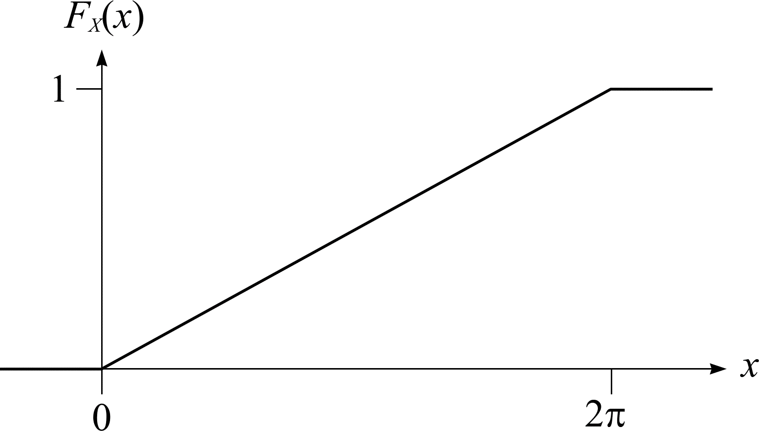
Figure 5: The distribution function \(F_{X}\) of \(X\) for the needle.