Vertical spatial grid
As shown in the previous section, the surface area, \(S\), of a bounded object, \(M\), can be estimated from two series of vertical sections (\(n = 2\)), separated by a distance \(T\), whose orientations are \(\phi_0 \in \mathrm{UR}[0, \pi /2)\) and \(\phi_1 = \phi_0 + \pi /2\). Let \(I_i\) be the number of intersections between the boundary of \(M\) on the sections of series \(i\) and the rolling cycloids. The surface area of \(M\) is given by
and from (49)
$$ S = \left(\frac{a}{l}\right) \cdot T \cdot \left(\mathbf{E}I_0 + \mathbf{E}I_1\right). \tag{50} $$
The vertical spatial grid (VSG), devised by Cruz-Orive and Howard (1995), is a test probe comprising two systems of rolling cycloids that allows the intersection counts \(I_0\) and \(I_1\) to be observed from a single series of vertical sections through \(M\). The rolling cycloids are contained in two mutually perpendicular sets of planes parallel to the sections in series 0 and series 1. Let series 0 be the observation series. The VSG, shown in Figure 23, consists of rolling cycloids parallel to the observation series that ride upon rolling cycloids normal to the observation series.
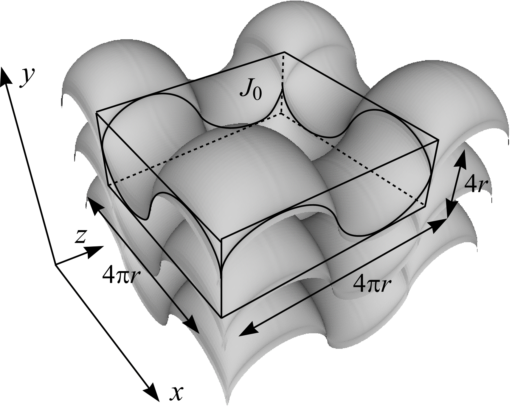
Figure 23: The vertical spatial grid and its fundamental tile, \(J_0\). The vertical spatial grid is a test probe comprising two systems of rolling cycloids that are contained in mutually orthogonal sets of planes (\(xy\) and \(yz\)). These systems of rolling cycloids sweep out the grey surface shown here.
Suppose a single (\(n = 1\)) observation series of \(m\) parallel vertical sections \((T_0, ..., T_{m-1})\) is constructed that cuts through \(M\) and whose orientation is \(\phi_0 \in \mathrm{UR}[0, \pi/2)\). As shown in Figure 24, let the distance between successive vertical sections be \(T\). On the first vertical section, \(T_0\), overlay a UR test system of points and rolling cycloids (see Figure 21(b)). Let \(I_{xy,0}\) be the number of intersections between the boundary of \(M\) on \(T_0\) and the rolling cycloids. Let \(P_0\) be the number of test points hitting the two dimensional cross-section of \(M\) on \(T_0\). Test points that contribute to \(P_0\) are considered "switched on" or highlighted.
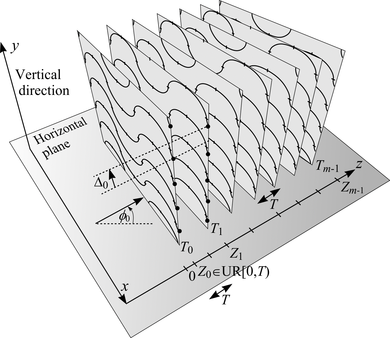
Figure 24: An observation series of \(m\) parallel vertical sections. The object of interest \(M\), through which the series cuts, is omitted for clarity.
On the second section, \(T_1\), of the observation series, overlay the same test system that appeared on \(T_0\), but shifted vertically by the signed distance \(\Delta_0\). The calculation of the vertical shift, \(\Delta_0\), is described below. In the same way as described in the previous paragraph, count \(I_{xy,1}\) and \(P_1\). On \(T_1\) (and subsequent sections) make an additional count \(P_{0,1}\) of highlighted points on \(T_0\) that remain highlighted on \(T_1\). Each of the three counts described is illustrated in Figure 25.
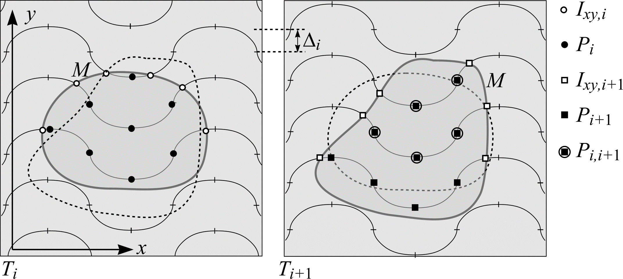
Figure 25: Point and intersection counting on the observation series. In this example, \(I_{xy,i} = 6\), \(P_i = 8\), \(I_{xy,i+1} = 6\), \(P_{i+1} = 9\) and \(P_{i,i+1} = 5\).
This process is repeated for all sections \(T_0, ..., T_{m-1}\) belonging to the observation series. The total number of intersections, \(I_0\), between the boundary of \(M\) on the observation series sections and the test systems of rolling cycloids is
$$ I_0 = \sum_{i=0}^{m-1} I_{xy, i}. $$
Consider a second constructed series of parallel vertical sections (shown in Figure 26), perpendicular to the observation series and horizontal plane, whose orientation is \(\phi_1 = \phi_0 + \pi/2\). Let the distance between successive vertical sections be \(\pi r\). Position the constructed series so that test points on the observation series also lie on the new series. The vertical shifts \(\Delta_i\) are calculated so that test points on the constructed series trace out constructed rolling cycloids that are normal to the observation series.
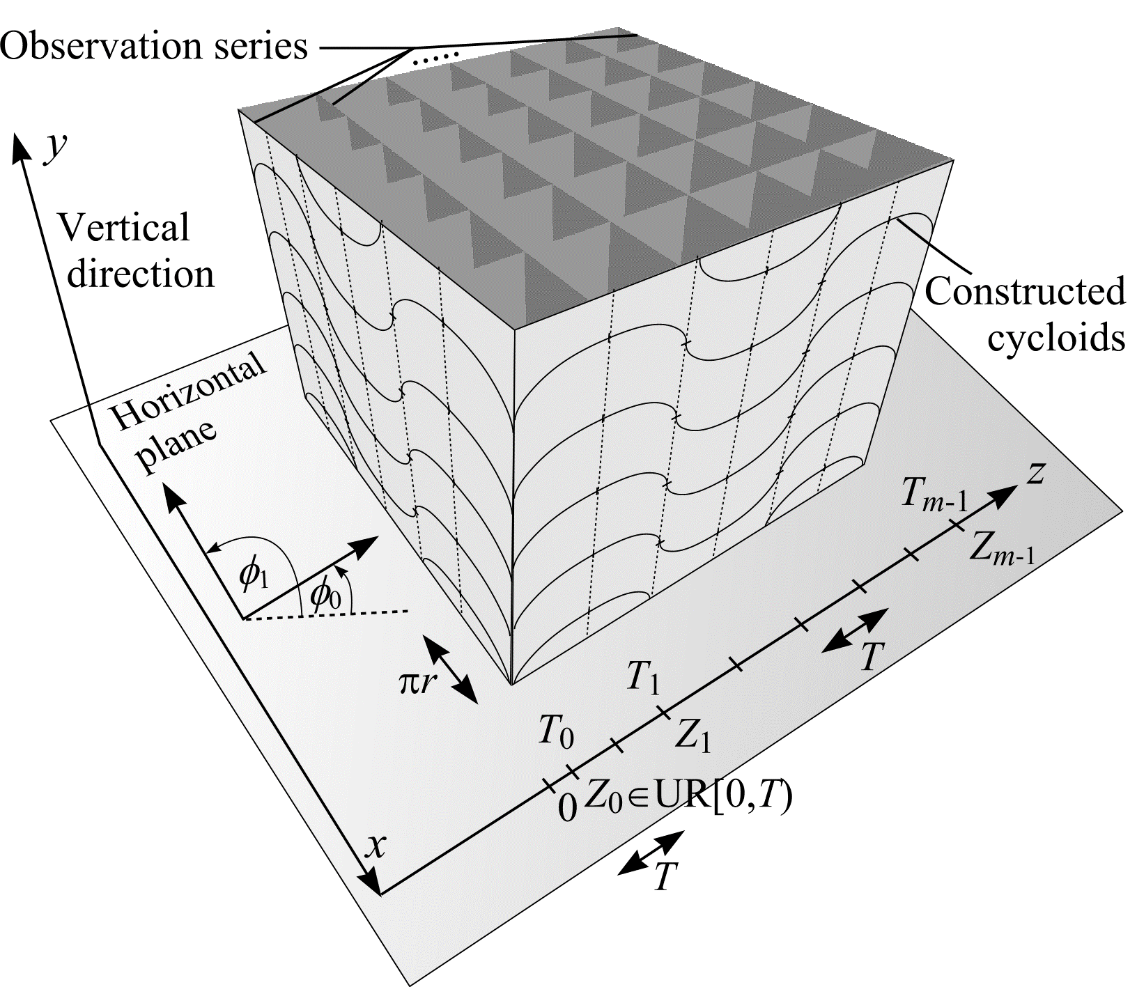
Figure 26: A constructed series of vertical sections perpendicular to the observation series. In this example, the distance between successive vertical sections on both series is \(\pi r\).
The vertical shifts \(\Delta_i\) are calculated as follows. Let \(Z_0 \in \mathrm{UR}[0, T)\) and \(Z_i = Z_0 + (i \cdot T)\) \((i = 0, ..., m - 1)\) be systematic abscissae along a rolling cycloid, radius \(r\), whose corresponding ordinates are \(Y_i\). As shown in Figure 27, the vertical shifts \(\Delta_i\) \((i = 0, ..., m - 2)\) are given by
$$ \Delta_i = Y_{i+1} - Y_{i} (i = 0, ..., m-2). $$
However, given a cycloid abscissa \(Z_i\), the corresponding ordinate \(Y_i\) is not available explicitly. (47) must be solved numerically for \(\theta\) and this value of \(\theta\) substituted into (48). For each \(i = 0, ..., m - 1\) let
$$ \theta_{i, 0} = \frac{Z_i}{r} $$
so that
$$ \theta_{i,k+1} = \sin\theta_{i,k} + \frac{Z_i}{r}, \text{(k = 0, 1, 2, ...).} $$
The solutions \(\theta_i\) are taken to be \(\theta_{i,N}\) as soon as \(| \theta_{i,N} - \theta_{i,N-1} | \lt \varepsilon\) or \(N \gt N_0\), where \(\varepsilon\) is a small positive number and \(N_0\) is the maximum number of iterations. Cruz-Orive and Howard (1995) suggest \(\varepsilon = 0.001\) and \(N_0 = 100\). Greater accuracy is readily achieved (by decreasing \(\varepsilon\) and increasing \(N_0\)) when modern computers are employed. Finally the solutions \(\theta_i\) are substituted into (48) to obtain \((i = 0, ..., m - 2)\)
$$ \Delta_i = \xi(\theta_{i+1}) - \xi(\theta_i) $$
where
$$ \xi(\theta) = \left((1 - \cos\theta)r\right) \cdot (-1)^{[\theta/(2\pi)]}. $$
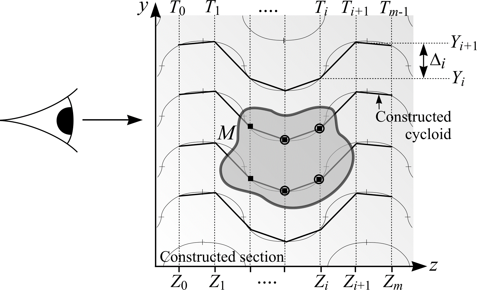
Figure 27: A constructed vertical section through \(M\). Test points on the observation series \(T_0, ...,T_{m-1}\) trace constructed rolling cycloids. Test points within \(M\) are represented by rectangles. Test points highlighted for more than one section (moving in the direction \(T_0\) to \(T_{m-1}\)) are circled. The number of intersections between the cross-section of \(M\) and the constructed rolling cycloids is \(I_1 = 2 \cdot (4 - 2) = 4\).
If a test point is highlighted on \(T_0\) and switched off on \(T_1\), then a constructed rolling cycloid has traversed the boundary of \(M\) (moving from the inside to the outside of \(M\)). For every inside-outside intersection, there must be a corresponding outside-inside intersection. Therefore, the total number of intersections, \(I_1\), between the boundary of \(M\) on the new series of sections and the constructed rolling cycloids is
$$ I_1 = 2 \cdot \left( \sum_{i=0}^{m-1} P_i - \sum_{i=0}^{m-2} P_{i,i+1} \right). $$
Equation (50) cannot be used directly to calculate the surface area of \(M\) when the VSG is employed. The extra constraints imposed on the positioning of the rolling cycloid test systems mean a new equation must be formulated. This is achieved by referring back to (45). If the boundary of \(M\) is intersected with an unbounded VSG then
$$ S = 2 \cdot \left( \frac{V}{\mathbf{E}L} \right) \cdot (\mathbf{E}I_0 + \mathbf{E}I_1). $$
\(L/V\) is the mean length of rolling cycloids per unit volume of space. As shown in Figure 24, the VSG has as its fundamental tile, \(J_0\), a rectangular box with volume \(V = 64 \pi r^3\). The mean length of rolling cycloid, \(\mathbf{E}L\), that falls within the volume is made up of two components.
The first component, \(\mathbf{E}L_0\), is the length of rolling cycloid contributed by the observation series. Each observation section that cuts through \(J_0\) contains one full period of rolling cycloid within \(J_0\). The expected number of observation sections that intersect \(J_0\) is \(4 \pi r/T\) - i.e., the length of \(J_0\) in the constructed series direction divided by the distance between observation series. Since one period of rolling cycloid has length \(16r\), \(\mathbf{E}L_0 = 16 r \cdot 4 \pi r / T = 64 \pi r^{2}/T\).
The second component, \(\mathbf{E}L_1\), is the length of constructed rolling cycloid contributed by the constructed series. Four constructed sections, a distance \(\pi r\) apart, cut through \(J_0\) and each section contains one full period of rolling cycloid within \(J_0\). Therefore \(\mathbf{E}L_1 = 4 \cdot 16r = 64r\), so that
$$ \begin{align} \frac{V}{\mathbf{E}L} &= \frac{64 \pi^2 r^3}{64r + \frac{64 \pi r^2}{T}} \\ &= \frac{\pi^2 r^2 T}{T + \pi r}. \end{align} \tag{51} $$
The rolling cycloids that comprise the VSG have test area per test point, \(a/p = \pi r \cdot 4r = 4 \pi r^2\) and test length per test point, \(l/p = 4r\). When these values are substituted into (51), Cruz-Orive and Howard's result for estimating surface area using the VSG is obtained:
Implementing the VSG is not straightforward. Some guidelines are stated here. Care should be taken to avoid periodicity between the step length \(T\) and the horizontal width of a cycloid, \(\pi r\), as this causes unwanted repetitions of the vertical shifts \(\Delta_i\) and decreases precision. Large values of \(T\) are also discouraged as this causes constructed cycloids (shown in Figure 27) to be poorly approximated and thus intersections contributing to \(I_1\) may be omitted.
Another issue is oversampling on either the observation series or the constructed series. This will occur if either VSG component (observed or constructed) has significantly greater length per unit volume (\(L/V\)) than the other. Figure 26 illustrates a VSG that has \(L/V\) identical for both components. The observation and constructed series intersect each other in a square lattice. Unfortunately, this configuration implies \(T = \pi r\) with unwanted repetitions of the vertical shifts \(\Delta_i\) resulting. These conflicting guidelines suggest the following VSG implementation:
Set \(T\) considerably smaller than \(\pi r\), e.g. \(T < \pi r/4\), (but not \(\pi r\) divided by some positive integer). Count intersections, \(I_1\), contributed by the constructed cycloids as described in the text. Intersections, \(I_0\), on the observation series should only be counted on every \([\pi r/T]^{\text{th}}\) section (where \([x]\) means the integer part of \(x\)). The distance between successive sections comprising the observation series is now \(T_2 = [\pi r/T] \cdot T\), and this value should be used instead of \(T\) in (52).
When the VSG is implemented using tools that allow vertical scanning, such as a confocal scanning laser microscope or a computer programme with 3D digital image loaded, the intersection count \(I_1\) need not be counted as described in the text. Instead virtual cycloid probes are imagined travelling normal to the observation series that pass through points on the observation cycloids (marked as vertical and horizontal lines in Figure 25).
Furthermore, 3D digital images can be reformatted using image analysis tools to produce 2D image sections that comprise observation and constructed series. For images sectioned in this way, true horizontal rolling cycloids can be overlain on both observation and constructed sections with intersection counts \(I_0\) and \(I_1\) recorded in the normal way.
References
CRUZ-ORIVE, L. M. and HOWARD, C. V. Estimation of individual feature surface area with the vertical spatial grid. J. Microsc., 178, 146-151 (1995).