IUR sections
In practice, surface density estimation is achieved by taking IUR sections through the object of interest, \(M\), and superimposing an IUR test system of lines onto each section. Subsequently, surface area may be calculated by multiplying the estimate of surface density by the reference volume, which may be obtained using the Cavalieri method.
An IUR section (or plane) in \(\real^{3}\) that cuts \(M\) is generated by the following procedure. Let \(u_{1} \in \mathrm{UR}[0, 1)\), \(u_{2} \in \mathrm{UR}[0, 1)\) and \(u_{3} \in \mathrm{UR}[0, 1)\) so that \(\theta = \cos^{-1}(1 - 2u_{1})\) and \(\phi = 2 \pi u_{2}\) define an isotropic orientation, \(\mathbf{n} \in \real^3\). Let \(h\) be the radius of a sphere that encompasses \(M\). As shown in Figure 18 the point \(\mathbf{a} \in \real^3\), found by moving a distance \(h \cdot u_{3}\) from the sphere's centre in the direction \(\mathbf{n}\), and the orientation \(\mathbf{n}\) together define an IUR plane in \(\real^3\) that may cut \(M\). If the plane misses \(M\), the procedure must be restarted with 3 new random numbers.
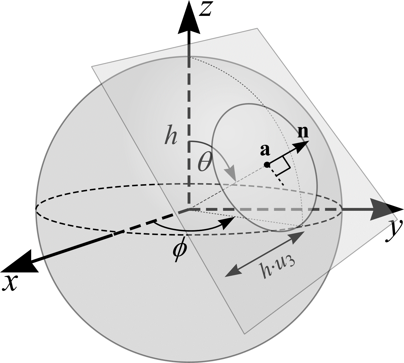
Figure 18: The construction of an IUR section.
When working with biological material it can be extremely cumbersome to generate IUR, physical sections. Mattfeldt et al. describe a way to generate IUR sections using the "orientator" (1990). Nyengaard and Gundersen (1992) describe an alternative approach using the "isector". However, non-invasive scanning techniques such as MRI enable a complete rendering of 3D structures, from which image analysis packages can generate IUR sections.
Given a set of IUR sections through \(M\), it is relatively easy to superimpose IUR test systems of lines onto each section. Generally, it is more efficient to superimpose IUR test systems comprising parallel or orthogonal lines. An IUR test system of orthogonal lines, a distance \(h\) apart, can be generated as follows. Let \(u_{1} \in \mathrm{UR}[0, 1)\), \(u_{2} \in \mathrm{UR}[0, 1)\), \(u_{3} \in \mathrm{UR}[0, 1)\) and \(\theta = 2 \pi u_{1}\). As shown in Figure 19(a), \(\mathbf{O} \in \real^2\) is a fixed origin on the IUR section and \(\theta\) is an angle relative to the fixed axis, \(O_x\). The points \(\mathbf{a}_{i}, \mathbf{b}_{i} \in \real^2\) \((-\infty < i < \infty)\) are found by moving, respectively, distances \(h \cdot u_{2} + i \cdot h\) and \(h \cdot u_{3} + i \cdot h\) from \(\mathbf{O}\) in the directions \(\theta\) and \(\theta + \pi / 2\). An IUR test system of orthogonal lines is constructed by drawing two sets of lines with orientations \(\theta + \pi/2\) and \(\theta\) through the points \(\mathbf{a}_{i}\) and \(\mathbf{b}_{i}.\)
Figure 19(b) shows an IUR section through an object \(M\) with an IUR test system of orthogonal lines overlain. The orthogonal grid of lines has 5 of its vertices within \(M\). The length of line, \(l\), and area, \(a\), associated with each vertex of the grid is \(l = 2h\) and \(a = h^{2}\). Therefore, an estimate of the length, \(L\), of test line falling within \(M\) is \(5\cdot 2 h = 10h\). The number of intersections, \(I\) = 10. The test system of orthogonal lines is said to have length per unit area \(l/a = 2/h\). A similar test system comprising a single set of parallel lines has length per unit area \(l/a = h/h^2 = 1/h\).
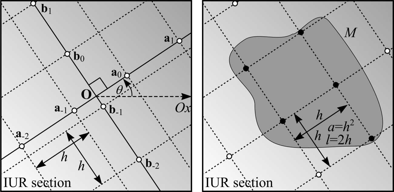
Figure 19: (a) The construction of an IUR test system of orthogonal lines. (b) The calculation of length per unit area, \(l/a\), for a test system of orthogonal lines.
Test systems of parallel and orthogonal lines are made up of test line elements that may be rearranged into any arbitrary curve shape whose mean length per unit area, \(l/a\), is known. Therefore, an alternative method is to overlay UR test systems of rolling circles (similar to that shown in Figure 13) on IUR sections through \(M\) and count intersections between the profile of \(M\) and the rolling circles. An estimate of the length, \(L\), of test line falling within \(M\) is obtained by counting points falling within \(M\) that are placed at quarter circle \((\pi r/2)\) intervals along each rolling circle.
References
MATTFELDT, T., MALL, G., GHAREHBAGHI, H. and MÖLLER, P. Estimation of surface area and length with the orientator. J. Microsc., 159, 301-317 (1990).
NYENGAARD, J. R. and GUNDERSEN, H. J. G. The isector: a simple and direct method for generating isotropic, uniform random sections from small specimens. J. Microsc., 165, 427-431 (1992).