Discrete random variables

The random variable \(X\) is discrete if it takes values in some countable subset \(\lbrace x_{1}, x_{2}, ...\rbrace\), only, of \(\real\). The distribution function of such a random variable has jump discontinuities at the values \(x_{1}, x_{2}\), ... and is constant in between. The function \(f_{X} : \real \to [0, 1]\) given by \(f_{X}(x) = \mathbf{P}(X = x)\) is called the (probability) mass function of \(X\). The mean value, or expectation, or expected value of \(X\) with mass function \(f_{X}\), is defined to be

$$ \begin{align} \mathbf{E}(X) &= \sum_{x} x f_{X}(x) \\ &= \sum_{x} x \mathbf{P}(X = x). \end{align} \tag{2} $$

The expected value of \(X\) is often written as \(\mu\).

It is often of great interest to measure the extent to which a random variable \(X\) is dispersed. The variance of \(X\) or \(\mathrm{Var}(X)\) is defined as follows:

$$\mathrm{Var}(X) = \mathbf{E}\left((X - \mathbf{E}(X))^{2} \right). \tag{3}$$

The variance of \(X\) is often written as \(\sigma^{2}\), while its positive square root is called the standard deviation. Since \(X\) is discrete, (3) can be re-expressed accordingly:

$$ \begin{align} \sigma^{2} &= \mathrm{Var}(X) \\ &= \mathbf{E}\left((X - \mu)^{2}\right) \\ &= \sum_{X}(x - \mu)^{2} f_{X}(x). \end{align} \tag{4} $$

In the special case where the mass function \(f_{X}(x)\) is constant and \(X\) takes \(n\) real values, (4) reduces to a well known equation determining the variance of a set of \(n\) numbers:

$$\sigma^{2} = \frac{1}{n}\sum_{X}(x - \mu)^{2}. \tag{5}$$

Events \(A\) and \(B\) are said to be independent if and only if the incidence of \(A\) does not change the probability of \(B\) occurring. An equivalent statement is \(\mathbf{P}(A \cap B) = \mathbf{P}(A)\mathbf{P}(B)\). Similarly, the discrete random variables \(X\) and \(Y\) are called independent if the numerical value of \(X\) does not affect the distribution of \(Y\). In other words, the events \(\lbrace X = x \rbrace\) and \(\lbrace Y = y \rbrace\) are independent for all \(x\) and \(y\). The joint distribution function \(F_{X, Y} : \real^{2} \to [0, 1]\) of \(X\) and \(Y\) is given by \(F_{X, Y}(x, y) = \mathbf{P}(X \le x \:\mathrm{and}\: Y \le y)\). Their joint mass function \(f_{X, Y} : \real^{2} \to [0, 1]\) is given by \(f_{X, Y}(x, y) = \mathbf{P}(X = x \:\mathrm{and}\: Y = y)\). \(X\) and \(Y\) are independent if and only if \(f_{X, Y}(x, y) = f_{X}(x)f_{Y}(y)\) for all \(x, y \in \real\).

Consider an archer, shooting arrows at the target shown in Figure 3. Suppose the archer is a very poor shot and hits the target randomly - in other words, target regions of equal area will have the same probability of being hit. For simplicity, it is assumed the archer always hits the target. If the archer is allowed to fire two arrows, the sample space

$$ \Omega = \begin{Bmatrix} \mathrm{AA}, & \mathrm{AB}, & \mathrm{AC}, & \mathrm{AD}, & \mathrm{AE}, \\ \mathrm{BA}, & \mathrm{BB}, & \mathrm{BC}, & \mathrm{BD}, & \mathrm{BE}, \\ \mathrm{CA}, & \mathrm{CB}, & \mathrm{CC}, & \mathrm{CD}, & \mathrm{CE}, \\ \mathrm{DA}, & \mathrm{DB}, & \mathrm{DC}, & \mathrm{DD}, & \mathrm{DE}, \\ \mathrm{EA}, & \mathrm{EB}, & \mathrm{EC}, & \mathrm{ED}, & \mathrm{EE} \\ \end{Bmatrix}. $$

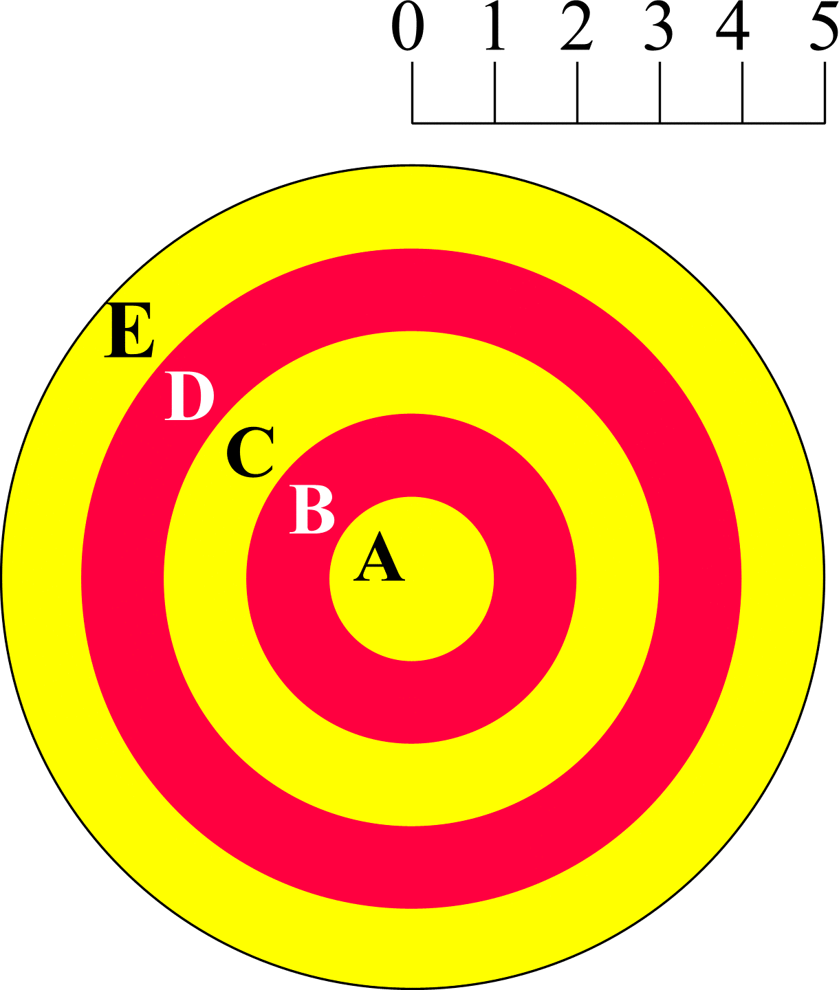
Figure 3: An archery target. A hit in region A scores 4 points, B scores 3 points, C scores 2 points, D scores 1 point and E scores nothing.

Let the variable \(X(\omega)\) represent the score of a particular outcome. The scoring guidelines outlined in Figure 3 imply \(X(\mathrm{AA}) = 8\), \(X(\mathrm{AB}) = X(\mathrm{BA}) = 7\), \(X(\mathrm{AC}) = X(\mathrm{BB}) = X(\mathrm{CA}) = 6\), ..., \(X(\mathrm{CE}) = X(\mathrm{DD}) = X(\mathrm{EC}) = 2\), \(X(\mathrm{DE}) = X(\mathrm{ED}) = 1\), \(X(\mathrm{EE}) = 0\). Clearly \(X\) is a discrete random variable, mapping the sample space \(\Omega\) to scores (real numbers).

The probability that an arrow hits a target region is directly proportional to the area of the region. The regions A to E are annuli with inner and outer radii as shown in Figure 3. The probabilities of hitting A to E are 1/25, 3/25, 5/25, 7/25 and 9/25 respectively. The mass function of \(X\), \(f_{X}(x)\), is then

$$ \begin{align*} f_{X}(0) &= \mathbf{P}(X = 0) \\ &= \mathbf{P}(\mathrm{Hit\:E})\mathbf{P}(\mathrm{Hit\:E}) \\ &= 81/625 \\ f_{X}(1) &= \mathbf{P}(X = 1) \\ &= 2 \cdot \mathbf{P}(\mathrm{Hit\:D})\mathbf{P}(\mathrm{Hit\:E}) \\ &= 126/625 \\ f_{X}(2) &= \mathbf{P}(X = 2) \\ &= \begin{align*}& 2 \cdot \mathbf{P}(\mathrm{Hit\:C})\mathbf{P}(\mathrm{Hit\:E}) \\ &+ \mathbf{P}(\mathrm{Hit\:D})\mathbf{P}(\mathrm{Hit\:D}) \end{align*} \\ &= 139/625 \end{align*} $$

and so on. From (2), the expected value of \(X\) is \(\mathbf{E}(X) = 0.81/625 + 1 \cdot 126/625 + 2 \cdot 139/625 + 3 \cdot 124/625 + ... = 2.4\). From (4), the variance of \(X\) is \(\mathrm{Var}(X) = 2.4^{2} \cdot 81/625 + 1.4^{2} \cdot 126/625 + 0.4^{2} \cdot 139/625 + 0.6^{2} \cdot 124/625 + ... = 2.72\). The distribution function of \(X\), \(F_{X}(x)\), is then

$$ \begin{align*} F_{X}(0) &= \mathbf{P}(X \le 0) \\ &= f_{X}(0) \\ F_{X}(1) &= \mathbf{P}(X \le 1) \\ &= f_{X}(1) + f_{X}(0) \\ F_{X}(2) &= \mathbf{P}(X \le 2) \\ &= f_{X}(2) + f_{X}(1) + f_{X}(0) \end{align*} $$

and so on. The distribution function \(F_{X}(x)\) is shown in Figure 4.

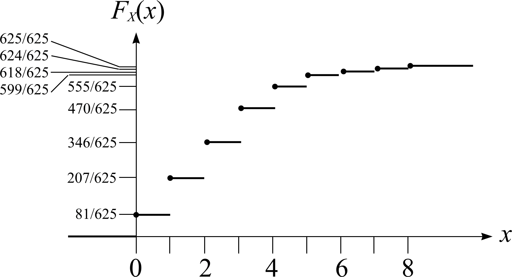
Figure 4: The distribution function \(F_{X}\) of \(X\) for the archery target.