Curve length in \(\real^{3}\)

In a previous section it is shown how Buffon's needle problem in two dimensions can be readily extended to facilitate calculation of curve length in \(\real^{2}\). In exactly the same way, Buffon's needle in three dimensions can be extended to estimate the length, \(L\), of a curve, \(C\), in \(\real^{3}\). The curve \(C\) is thrown isotropic uniform randomly into the array of planes.

Suppose the curve \(C\) is approximated by a union of line segments, \(Y = \bigcup(y_{i})_{i=1}^{n} = \{y_{1}, y_{2}, ..., y_{i}, ..., y_{n}\}\). If the length of \(y_{i}\) is \(l_{i}\) \((1 \le i \le n)\), an approximation of the curve length of \(C\) is \(L = \sum_{i=1}^{n} l_{i}\). By comparison with (38), the probability that the line segment \(y_{i}\) intersects a joint is \(l_{i}/2h\). Furthermore, (39) implies the length of \(y_{i}\) is \(l_{i} = 2 h \mathbf{E}Q_{i}\). \(Q_{i}\) is a discrete random variable that maps the outcomes \(y_{i}\) transects a plane and \(y_{i}\) falls between planes to the real numbers 1 and 0, respectively. Let the total number of transects, \(Q\), between the planes and \(Y\) be denoted as the sum \(Q_{1} + Q_{2} + ... + Q_{n}\). Taking into account all line segments:

$$ \begin{align} L &= 2 \cdot h \cdot \sum_{i=1}^{n} \mathbf{E}Q_{i} \\ &= 2 \cdot h \cdot \sum_{i=1}^{n} \mathbf{E}Q. \end{align} \tag{41} $$

An estimate of \(L\) can be obtained from a single throw of \(Y\). An estimate of \(L\) is

$$ \begin{align} \hat{L} &= 2 \cdot h \cdot \sum_{i=1}^{n} Q_{i} \\ &= 2 \cdot h \cdot Q. \end{align} \tag{42} $$

Finally, consider again the systematic set of parallel planes a distance \(h\) apart. The average area of test plane likely to fall within a certain volume can be calculated. Figure 15(a) shows an area of test plane, \(A\), and the volume it occupies. The test system of planes has area per unit volume \(A/V = A/Ah = 1/h\). Next, substitute \(h = V/A\) into (41). The result is an important formula originally due to Saltykov (1946):

$$ \begin{align} \frac{L}{V} &= 2 \cdot \frac{\mathbf{E}Q}{A} \\ \text{and so } L &= 2 \cdot \frac{V}{A} \cdot \mathbf{E}Q. \end{align} \tag{43} $$

An estimate of \(L\) can be obtained from a single throw of \(Y\):

$$ \hat{L} = 2 \cdot \frac{V}{A} \cdot Q. \tag{44} $$

Suppose a needle, length \(L\) \((L > h)\), is thrown with IUR position onto a test system of parallel planes. \(\hat{L}\) is greatest when the needle is perpendicular to the test planes and smallest when the needle is parallel to the test planes. A better estimation of \(L\) is obtained if the test system of parallel planes is replaced by a test system of three sets of mutually orthogonal planes (see Figure 15(b)). Such a test system has three times as much area per unit volume as the parallel plane test system so that \(A/V = 3 \cdot (1/h)\).

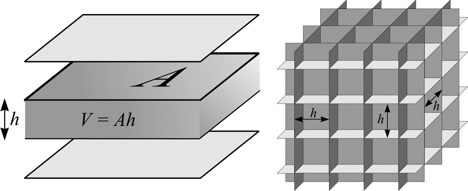
Figure 15: Test systems of (a) parallel planes (\(A/V = 1/h\)) and (b) mutually orthogonal planes (\(A/V = 3/h\)). The figure shows each test system with the volume, \(V\), an area of test surface, A, occupies.

References

SALTYKOV, S. A. The method of intersections in metallography (In Russian). Zavodskaja laboratorija, 12, 816-825 (1946).